Quick Note
Though they are not strictly connected, I recommend viewing the 4 sections in order to know how to not only train a model, but to make your own custom training procedure.
Though they are not strictly connected, I recommend viewing the 4 sections in order to know how to not only train a model, but to make your own custom training procedure.
Importing batch_norm would also recursively import all of it's dependencies. Reducing the need of having many import statements.
from batch_norm import *Building a model is incredibly simple. The comments in the snippet are the output dimensions of each layer for clarity. Now that we have a model, it will be used in the two final sections of this demo.
model = Sequential(Reshape((1, 28, 28)),
                   Conv(c_in=1, c_out=4, k_s=5, stride=2, pad=1), # 4, 13, 13
                   AvgPool(k_s=2, pad=0), # 4, 12, 12
                   BatchNorm(4),
                   Conv(c_in=4, c_out=16, stride=2, leak=1.), # 16, 5, 5
                   BatchNorm(16),
                   Flatten(),
                   Linear(400, 64), # 16 * 5 * 5 -> 400
                   ReLU(),
Linear(64, 10, True))Custom __repr__ methods let classes to be neatly displayed. It also works for nested models as shown in this notebook.
modelPrinting out parameters' information is also useful for debugging. Here is how to print out all model parameters.
for p in model.parameters():
print(p)If you want to only look into a selected layer, here it is how.
print(f'layer2: {model.layers[1]}\n')
for p in model.layers[1].parameters():
print(p)from callback import *I decided to use LearningRateSearch as our example since it will be used in the next section of this demo. As shown, before each batch, the callback would try a new learning rate while keeping track of the best learning rate (measured by loss) so far and automatically stop training after loss increases 10x or we have tried enough learning rates.
class LearningRateSearch(Callback):
    def __init__(self, max_iter=1000, min_lr=1e-4, max_lr=1):
        self.max_iter = max_iter # max number of candidates learning rates to try
        self.min_lr = min_lr  # lowest/starting candidate learning rate
        self.max_lr = max_lr  # highest candidate learning rate
        self.cur_lr = min_lr  # current candidate learning rate holder
        self.best_lr = min_lr # recorded learning rate with the lowest loss
        self.best_loss = float('inf') # lowest loss so far

    def before_batch(self):
        # assert training state
        if not self.model.training: return
        # calculate new candidate learning rate
        position = self.iters_count / self.iters
        self.cur_lr = self.min_lr * (self.max_lr/self.min_lr)**position
        # set learning rate in optimizer
        self.optimizer.hyper_params['learning_rate'] = self.cur_lr

    def after_step(self):
        # stop when either tried enough times or loss starts increasing
        if self.iters_count >= self.max_iter or self.loss > self.best_loss*10:
            raise CancelTrainException()
        # update best loss and best learning rate
        if self.loss < self.best_loss:
            self.best_loss = self.loss
self.best_lr = self.cur_lrfrom stateful_optim import *Let's retrieve the data bunch and loss function each using just one line. Since we are training on MNIST handwritten digits, cross entropy is an appropriate loss function to use.
data_bunch = get_data_bunch(*get_mnist_data(), batch_size=64)
loss_fn = CrossEntropy()model = get_conv_final_model(data_bunch)
optimizer = adam_opt(model, learning_rate=1e-3, weight_decay=1e-4)
callbacks = [LearningRateSearch(min_lr=1e-5, max_lr=1e-2), Recorder()]For model training, the best practice is to throw all components from above into a learner class, which is able to interact with callbacks in various stages of training.
By printing out the learner class, again with custom __repr__, we can view details on the data bunch, model architecture, loss function, optimizer steppers, and callbacks.
learner = Learner(data_bunch, model, loss_fn, optimizer, callbacks)
print(learner)To find our learning rate, simply do a 1 epoch fit. Recall from Making a Callback that the LearningRateSearch callback performs early stopping once it is confident in having the learning rate that yields the lowest loss.
learner.fit(1)By passing the Recorder callback into the util function plot_lr_loss, we can see the relationship between loss vs. learning rate.
plot_lr_loss(learner.callbacks[2])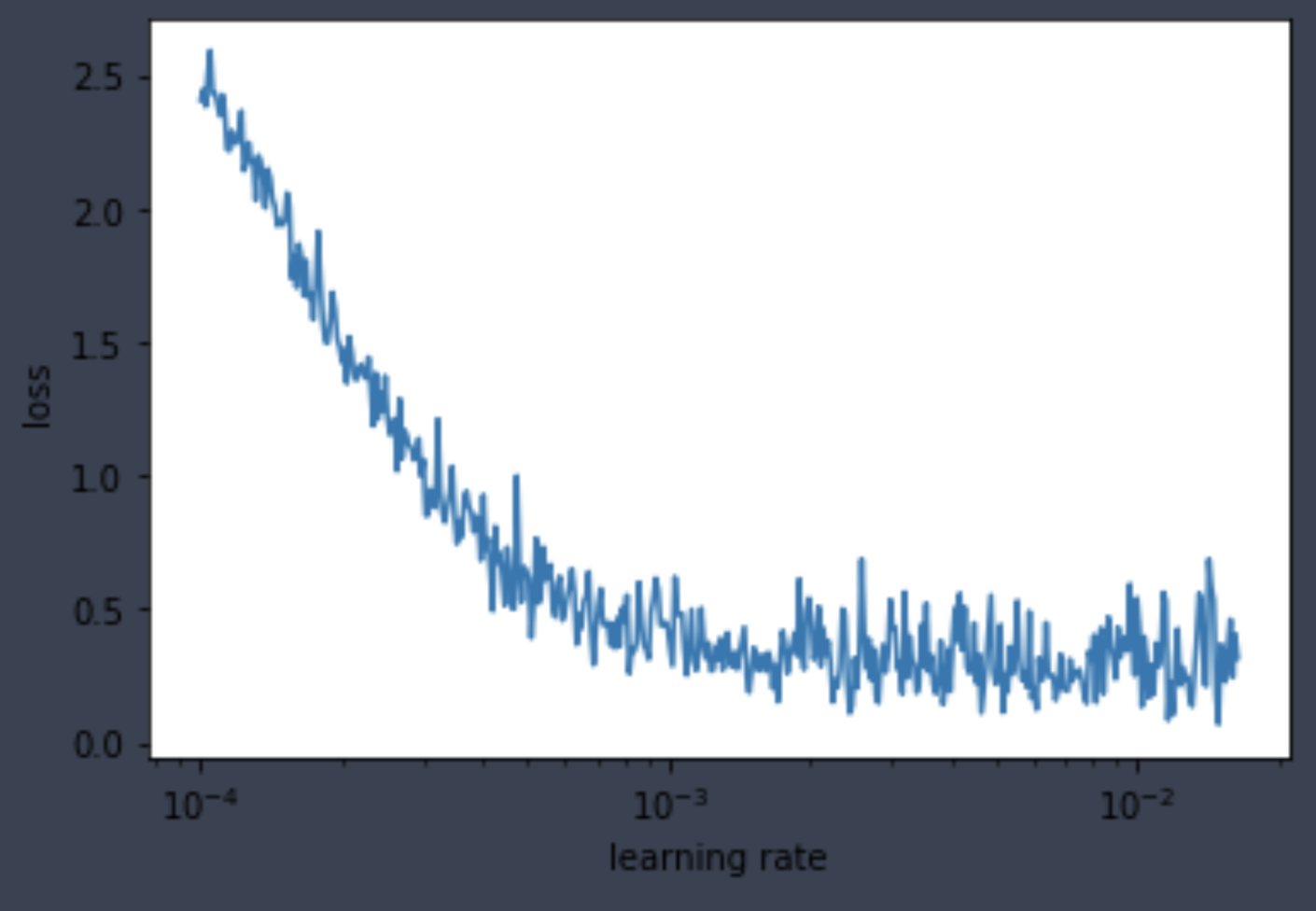
Lastly, the LearningRateSearch callback also kept track of the best learning rate candidate for our use in the final section.
lr = learner.callbacks[1].best_lr
print(f'learning rate found: {lr}')Same as previous sections, import modules, then grab data bunch and loss function.
from stateful_optim import *data_bunch = get_data_bunch(*get_mnist_data(), batch_size=64)
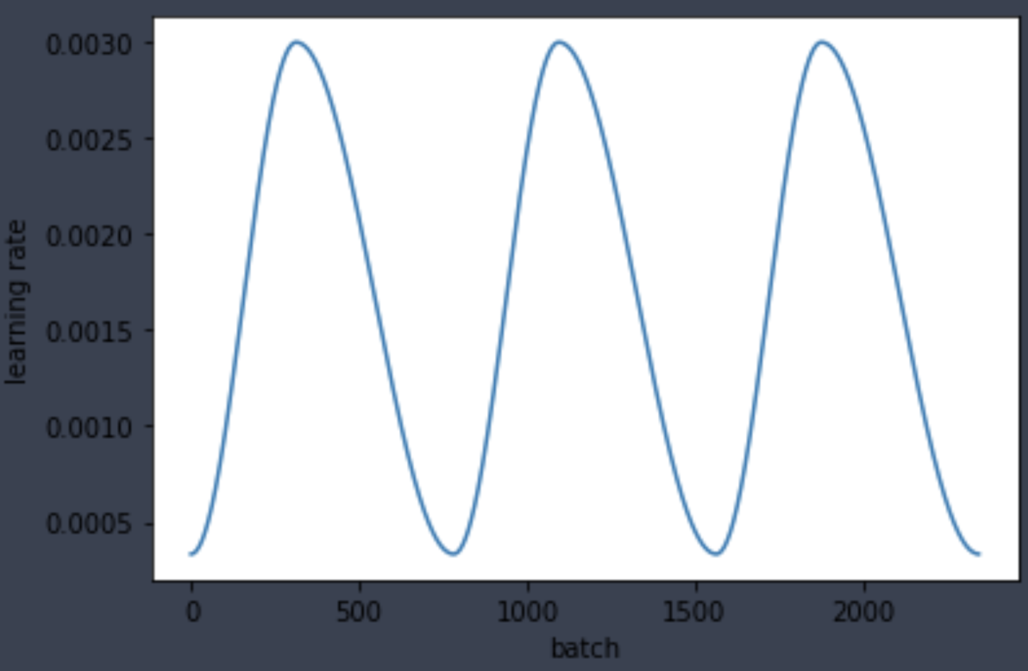
loss_fn = CrossEntropy()New callback alert! Please refer to the code documentation to familiarize with the ParamScheduler callback. Here we build a custom cosine schedule for the learning rate that takes place each epoch using the learning rate from the last section.
schedule = combine_schedules([0.4, 0.6], one_cycle_cos(lr/3, lr*3, lr/3))Same as before, create model, optimizer, and callbacks. Notice that LearningRateSearch is no longer needed and that the ParamScheduler is now used for training with dynamic learning rate per epoch. I also added StatsLogging to print out loss and accuracy per epoch.
model = get_conv_final_model(data_bunch)
optimizer = adam_opt(model, learning_rate=lr, weight_decay=1e-4)
callbacks = [ParamScheduler('learning_rate', schedule), StatsLogging(), Recorder()]
learner = Learner(data_bunch, model, loss_fn, optimizer, callbacks)
print(learner)Training is as simple as just calling the fit method with number of epochs. As shown below, the validation accuracy rises to 97.3 in just 3 epochs.
learner.fit(3)Lastly, plot the loss and learning rate recorded by the Recorder callback.
learner.callbacks[3].plot_losses()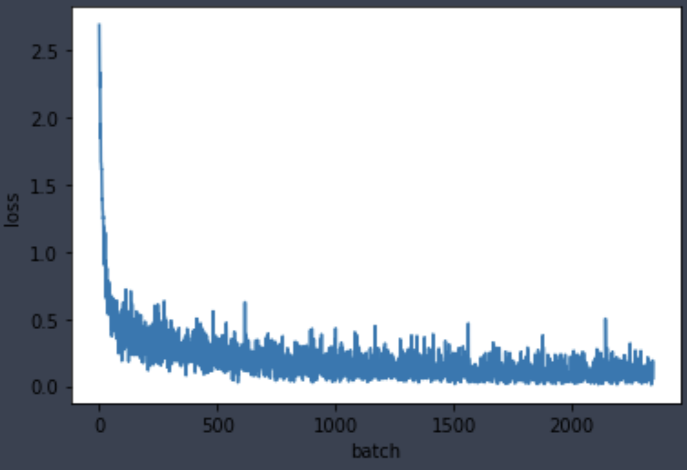
As shown below, the learning rate values make a cosine-ish cycle each epoch, showing that our ParamScheduler callback is working properly.
learner.callbacks[3].plot_parameter('learning_rate')